7. Project: Newton’s Divided Difference Interpolation#
7.1. Introduction#
In this project, you will write a MATLAB code to calculate the set of divided differences and use it to calculate the Newton divided difference form of the interpolation polynomial. To get started with this project, you will need to download the starter code and unzip its contents to the directory where you wish to complete the project.
Files included in this project
project7.m - MATLAB script that steps you through the project.
checkMyAnswer.m - MATLAB script that checks your code.
checkMyAnswer.mat - Data set.
data.mat - Data set.
* divdif.m - Divided difference of the function.
* interp.m - Newton divided difference form of the interpolation polynomial.
You need to complete the files with *.
Throughout the project, you will be using the script project7.m. This script set up all dataset for the problem and make calls to functions that you will write. Do not modify it. You are only required to modify functions in * files, following the instructions in this project.
7.2. Assignments#
Part 1 - Divided Difference#
The first part of project7.m gives you practice with evaluating
divided differences in MATLAB. Recall divided differences are
Note however that MATLAB does not allow zero subscripts, we should rewrite above formula as
In the file divdif.m, you will find the outline of a MATLAB
function. Modify it to return the vector \([D_1,D_2,...D_m]\).
Hint
Use this table to find the general pattern of D(i) in stage k.
\(i\) |
\(x_i\) |
\(f[x_i]\) |
\(f[x_{i-1},x_i]\) |
\(f[x_{i-2},x_{i-1},x_i]\) |
\(f[x_{i-3},x_{i-2},x_{i-1},x_i]\) |
|---|---|---|---|---|---|
1 |
\(x_1\) |
\(f(x_1)\) |
|||
2 |
\(x_2\) |
\(f(x_2)\) |
\(\dfrac{f[x_2]-f[x_1]}{x_2 - x_1}\) |
||
3 |
\(x_3\) |
\(f(x_3)\) |
\(\dfrac{f[x_3]-f[x_2]}{x_3 - x_2}\) |
\(\dfrac{f[x_2,x_3]-f[x_1,x_2]}{x_3 - x_1}\) |
|
4 |
\(x_4\) |
\(f(x_4)\) |
\(\dfrac{f[x_4]-f[x_3]}{x_4 - x_3}\) |
\(\dfrac{f[x_3,x_4]-f[x_2,x_3]}{x_4 - x_2}\) |
\(\dfrac{f[x_2, x_3,x_4]-f[x_1,x_2,x_3]}{x_4 - x_1}\) |
Now you can run project7.m and it will show you the points used in
this project by table and scatter plot. Then you should see the first
four divided differences are:
=============================================
The first four divided differences are:
==
==  i |     D_i
== -- | -------
==  0 |  1.0000
==  1 | -0.0995
==  2 | -0.4887
==  3 |  0.0479
== -------------
=============================================
Part 2 - Polynomial interpolation in Newton’s form#
In this part of project, you will complete the code in interp.m to
calculate the Newton divided difference form of the interpolation
polynomial. Recall the Newton divided difference interpolation formula
is
However, as mentioned above, MATLAB does not allow zero subscripts, so we rewrite the formula as
Hint
You can use a two-level nested for loop to implement this formula.
Use the inner
forloop to calculate the product, sayp, in thekterm: \((x-x_1)(x-x_2)\cdots(x-x_{k-1})\).Use the outer
forloop to sum upD(k)*p.
Now you can run project7.m and it will show you the evaluations of y
at some values of x. You will see the following output:
=============================================
The evaluation of y at x=0.15 is -27.0758
The evaluation of y at x=1.23 is  0.3339
The evaluation of y at x=2.66 is -0.8863
The evaluation of y at x=6.19 is  3.9921
=============================================
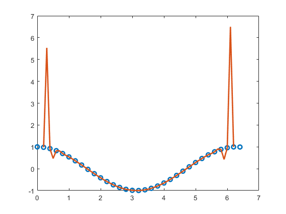
and the following graph:

The blue circles represent the points given and the red line represents the interpolation plynomial by Newton divided difference. You can see that the interpolation evaluates well for the interiors, but badly for the region near the endpoints. This is called Runge’s phenomenon. We will learn cubic spline interpolation to avoid this phenomenon next week.
7.3. Submit your code#
This is the last step. You should submit your code files to WTClass. After clicking Browse My Computer, you should select all files listed in Introduction to upload. Failure to do so will affect your grade.