

|
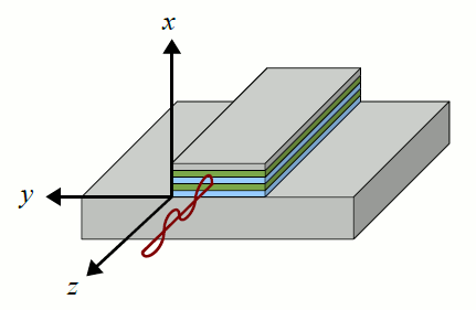
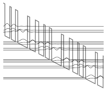
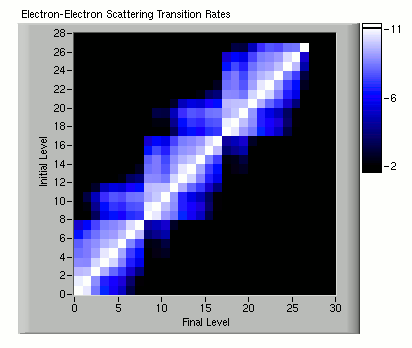
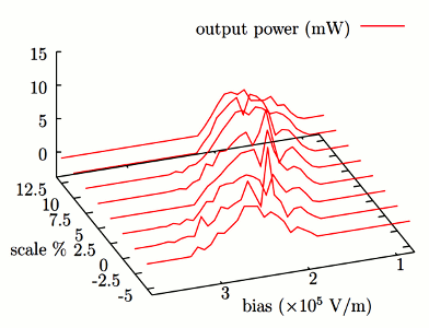
Code Overview This is a diagram illustrating how all the pieces below fit together. It lists the equations that need to be solved, where they are best solved, and the structure of the self-consistent loops. 1. Find Initial Effects1.1 Create Location GridCreate the grid of spatial points on which all else will be calculated. Defining at the start a standard grid of points that all calculations will use enables efficient development and minimization of error. A typical QCL is homogenous in the transverse directions, so that the grid need only span the z dimension. A grid with non-uniform step sizes is used to ensure that material layer widths are preserved exactly.  Calculate waveguide loss and mode confinement as a function of frequency using a slab model. The modes of the user-defined waveguide are found using the transfer matrix approach and a gradient descent search of the space of all possible complex wavenumbers until converging on the possible modes. For the purposes of the waveguide calculations, the active region is treated as one homogenous layer with an average doping. 1.3 Space Charge Density Model the electron space charge initially as a bunch of charge behind the injection barrier, then find it as populations times wavefunctions.The space charge is a sum of the conduction electron spatial density and the fixed ionized donor density. The space charge gives rise to the built-in electrostatic potential which effects the electron wavefunctions according to the Schroedinger equation. 2. Find Wavefunctions2.1 Poisson EquationSolve the 1D poisson equation as a function of space charge using the Runge-Kutta 4th order method. The material permittivity is not spatially uniform, but depends on the z dimension, and therefore cannot be moved out of the derivatives.  Calculate the total potential as the conduction band edge profile plus the built-in voltage plus the applied bias. 2.3 Schroedinger Equation Solve the 1D Schroedinger equation as a function of the total potential using the Runge-Kutta 4th order method.The material permittivity is not spatially uniform, but depends on the z dimension, and therefore cannot be moved out of the derivatives. The eigenenergies are found by calculating an initial sweep of energies, identifying those energies in the sweep that give the lowest error, and refining those energies using a binary search of the error space. The wavefunctions are calculated accross three periods of the QCL structure with Dirichlet boundary conditions. The wavefunctionsin the inner period are then copied to the outer periods to ensure pseudo-periodicity. 2.4 Copy Wavefunctions Copy wavefunctions in the central period to the outer periods to ensure perfect pseudo-periodicity. Although wavefunctions span several periods, their center-of-masses are calculated and the wavefunctions are assigned to a period depending on the location of their center-of-masses. 3. Find Scattering Rates3.1 Individual Fermi LevelsFind the subband-specific Fermi levels as a function of temperature and population for use in the scattering calculations. All subbands are assumed to be constantly thermalized into Fermi distributions, each with its own temperature and Fermi level describing the distribution.  Calculate electron-electron scattering rates using Fermi's golden rule with a Coulomb-like Hamiltonian. State blocking is neglected as it was found to be negligible. Screening effects are included. We sum over all possible final wavevectors and average over all possible initial wavevectors. The form factor is pre-calculated as a look-up table. 3.3 Electron-Electron Screening Calculate electron-electron screening using the self-consistent field model. 3.4 Phonon Scattering Calculate the LO phonon scattering rates using Fermi's golden rule and the Froehlich interaction. 3.5 Photon Scattering Calculate the photon scattering rates using Fermi's golden rule and the electron-photon field interaction Hamiltonian. 4. Find Populations and Power4.1 Rate EquationsSolve the all-electron-levels/all-photon-levels coupled rate equations to find all electron and photon populations.  Calculate the laser output power as the photon population times the energy per photon times the front facet emission rate. |